Chapter 1 — Fundamental Concepts¶
1.8 — Analytic Geometry¶
Analytic geometry translates figures into equations, and equations into figures: it is a dictionary between two languages that say the same thing.
Until now all the geometry in this book has lived in a single dimension: the real line, with the distance of §1.1 that we used in the inequalities of §1.7. This section takes the step to two dimensions. Each point of the plane will be described by a pair of real numbers, and with that, geometric figures can be described by equations. This is the idea of Descartes and Fermat in the seventeenth century: a circle, which for Euclid was a figure, also becomes the solution set of an equation, and geometric questions become algebraic questions.
§1. The Cartesian plane¶
An ordered pair \((a, b)\) is a pair of numbers in which order matters: \((a, b) = (c, d)\) means that \(a = c\) and \(b = d\). Thus \((1, 2)\) and \((2, 1)\) are different pairs. The set of all ordered pairs of real numbers is denoted \(\mathbb{R}^2\):
To give \(\mathbb{R}^2\) a geometric picture, we draw in the plane two perpendicular lines, each with its scale of real numbers like the line of §1.1: the \(x\)-axis, horizontal, and the \(y\)-axis, vertical. They meet at the origin, which corresponds to the \(0\) of both. Through each point \(P\) of the plane we draw the perpendicular to the \(x\)-axis and the perpendicular to the \(y\)-axis. The numbers those perpendiculars mark on each axis are the coordinates of \(P\): the first, \(x\), is called the abscissa, and the second, \(y\), the ordinate, and we write \(P = (x, y)\). Conversely, each pair \((x, y)\) determines a unique point. This correspondence between points and pairs is the starting point of analytic geometry: from here on, we identify the plane with \(\mathbb{R}^2\) and speak interchangeably of the point or the pair.
The axes divide the rest of the plane into four regions, the quadrants, numbered counterclockwise starting from the one containing the points with both coordinates positive. Points lying on the axes belong to no quadrant.
Reminder. A point of the plane is an ordered pair \((x, y)\) of real numbers; \((a, b) = (c, d)\) means \(a = c\) and \(b = d\).
§2. The distance between two points¶
On the line, §1.1 defined the distance between \(a\) and \(b\) as \(|b - a|\). In the plane, distance is obtained by combining that idea with the Pythagorean theorem of Euclidean geometry.
Proposition. The distance between \(P_1 = (x_1, y_1)\) and \(P_2 = (x_2, y_2)\) is
Proof. Let us begin with a fact about real numbers: for every real \(u\), \(\sqrt{u^2} = |u|\). Indeed, \(|u|\) is nonnegative and its square is \(u^2\), because \(|u|\) is \(u\) or \(-u\) and \((-u)^2 = u^2\); by the uniqueness of the root in §1.2, \(|u|\) is the square root of \(u^2\).
If \(y_1 = y_2\), the two points lie on the same horizontal line and their distance is the distance between their abscissas, \(|x_2 - x_1|\). The formula gives \(\sqrt{(x_2 - x_1)^2} = |x_2 - x_1|\), and they agree. The case \(x_1 = x_2\) is analogous. In the general case, consider the auxiliary point \(Q = (x_2, y_1)\). The segment \(P_1Q\) is horizontal and measures \(|x_2 - x_1|\); the segment \(QP_2\) is vertical and measures \(|y_2 - y_1|\). Since they are perpendicular, \(P_1\), \(Q\) and \(P_2\) form a right triangle whose hypotenuse is \(P_1P_2\), and by the Pythagorean theorem,
The right-hand side is nonnegative, because it is a sum of squares, and so is the distance; by the uniqueness of the root, \(d(P_1, P_2)\) is the square root of the right-hand side. \(\blacksquare\)
The proof uses a theorem of Euclidean geometry, the Pythagorean theorem, which does not follow from the axioms of \(\mathbb{R}\). For that reason, from here on we adopt the formula as the definition of distance in \(\mathbb{R}^2\). The proposition guarantees that this definition agrees with the distance of Euclidean geometry, and from now on all proofs about distances in the plane will be algebraic.
Example. The distance between \((1, -2)\) and \((4, 2)\) is \(\sqrt{(4 - 1)^2 + (2 - (-2))^2} = \sqrt{9 + 16} = 5\).
Reminder. \(d(P_1, P_2) = \sqrt{(x_2 - x_1)^2 + (y_2 - y_1)^2}\): the Pythagorean theorem applied to the differences of coordinates.
§3. The midpoint¶
The midpoint of the segment joining \(P_1 = (x_1, y_1)\) and \(P_2 = (x_2, y_2)\) is the point of the segment at the same distance from both endpoints. Its coordinates are the averages of the coordinates of the endpoints.
Proposition. Let \(M = \left(\dfrac{x_1 + x_2}{2}, \dfrac{y_1 + y_2}{2}\right)\). Then
Proof. The differences of coordinates between \(P_1\) and \(M\) are \(\frac{x_1 + x_2}{2} - x_1 = \frac{x_2 - x_1}{2}\) and, likewise, \(\frac{y_2 - y_1}{2}\). By the formula of §2,
where we used that \(\sqrt{\frac{s}{4}} = \frac{\sqrt{s}}{2}\) for \(s \ge 0\), by the quotient property of radicals in §1.2. The differences between \(M\) and \(P_2\) are \(\frac{x_2 - x_1}{2}\) and \(\frac{y_2 - y_1}{2}\), the same ones, so \(d(M, P_2)\) gives the same value. \(\blacksquare\)
The proposition says that \(M\) is equidistant from \(P_1\) and \(P_2\), and that \(d(P_1, M) + d(M, P_2) = d(P_1, P_2)\). In Euclidean geometry, the points whose distances to the endpoints add up exactly to the length of the segment are the points of the segment; therefore \(M\) lies on the segment and is its midpoint.
Example. The midpoint of the segment joining \((1, -2)\) and \((4, 2)\) is \(\left(\frac{5}{2}, 0\right)\), and its distance to each endpoint is \(\frac{5}{2}\), half of \(5\).
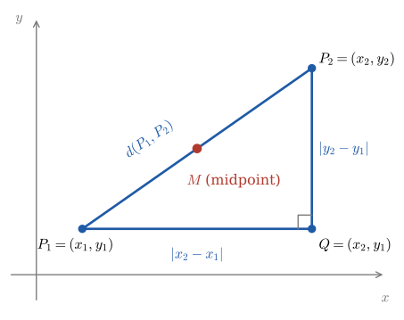
Figure 1.4 — The right triangle \(P_1QP_2\) from the proof in §2, with the midpoint \(M\) of §3 marked on the hypotenuse.
Reminder. The midpoint has as coordinates the averages of the coordinates of the endpoints, and it lies at half the distance from each one.
§4. The circle¶
A circle with center \((h, k)\) and radius \(r > 0\) is the set of points of the plane at distance exactly \(r\) from the center. With the formula of §2, that geometric definition becomes an equation.
Proposition (standard equation of the circle). A point \((x, y)\) belongs to the circle with center \((h, k)\) and radius \(r\) if and only if
Proof. By definition, \((x, y)\) belongs to the circle if and only if \(d\big((x, y), (h, k)\big) = r\), that is, \(\sqrt{(x - h)^2 + (y - k)^2} = r\). By the proposition of §1.5 on equations with radicals, this equality holds if and only if \((x - h)^2 + (y - k)^2 = r^2\) and \(r \ge 0\). Since \(r > 0\), the second condition always holds, and the equation in the statement remains. \(\blacksquare\)
Here squaring adds no solutions, and §1.5 says why: the right-hand side, \(r\), is not negative.
Often the equation does not appear in its standard form but expanded, as \(x^2 + y^2 + Dx + Ey + F = 0\). To recover the center and the radius we complete the square, as in §1.3, once in each variable. Since \(x^2 + Dx = \left(x + \frac{D}{2}\right)^2 - \frac{D^2}{4}\), and likewise with \(y\), the equation is equivalent to
Not every equation of this form is a circle. Let us call \(c\) the number on the right-hand side. If \(c > 0\), the equation is that of the circle with center \(\left(-\frac{D}{2}, -\frac{E}{2}\right)\) and radius \(\sqrt{c}\). If \(c = 0\), a sum of two squares is zero only if both are zero, because each is nonnegative (§1.3), and the only point satisfying it is \(\left(-\frac{D}{2}, -\frac{E}{2}\right)\). If \(c < 0\), no point satisfies it, because a sum of squares is not negative.
Example. Consider \(x^2 + y^2 - 6x + 4y + 9 = 0\). Grouping and completing the square in each variable,
The right-hand side is positive: the equation is that of the circle with center \((3, -2)\) and radius \(\sqrt{4} = 2\). On the other hand, \(x^2 + y^2 - 6x + 4y + 14 = 0\) leads to \((x - 3)^2 + (y + 2)^2 = -1\), which has no solution at all.
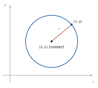
Figure 1.5 — Circle with center \((h,k)\) and radius \(r\): "distance to the center equals \(r\)" written in symbols.
Reminder. \((x - h)^2 + (y - k)^2 = r^2\) is "distance to the center equals \(r\)" written in symbols. The general form is brought to standard form by completing the square, and it is a circle only if the right-hand side turns out positive.
§5. Symmetry¶
We call a curve the set of points \((x, y)\) of the plane that satisfy an equation in \(x\) and \(y\); the graph of the equation. A curve is symmetric with respect to the \(y\)-axis if, for each point \((x, y)\) of the curve, \((-x, y)\) also lies on it. It is symmetric with respect to the \(x\)-axis if, for each \((x, y)\), \((x, -y)\) also lies on it, and symmetric with respect to the origin if \((-x, -y)\) does. Geometrically, \((-x, y)\) is the reflection of \((x, y)\) in the \(y\)-axis, \((x, -y)\) its reflection in the \(x\)-axis, and \((-x, -y)\) the opposite point through the origin.
These conditions are checked with algebra. The point \((-x, y)\) satisfies the equation of the curve exactly when \((x, y)\) satisfies the equation that results from replacing \(x\) by \(-x\). Therefore, if that replacement yields an equation equivalent to the original, the curve is symmetric with respect to the \(y\)-axis. Likewise, replacing \(y\) by \(-y\) decides symmetry with respect to the \(x\)-axis, and replacing both at once, symmetry with respect to the origin.
Examples. In \(y = x^2\), replacing \(x\) by \(-x\) gives \(y = (-x)^2 = x^2\), the same equation: the curve is symmetric with respect to the \(y\)-axis. In \(y = x^3\), replacing \(x\) by \(-x\) and \(y\) by \(-y\) gives \(-y = -x^3\), which is equivalent to \(y = x^3\): the curve is symmetric with respect to the origin. The circle \(x^2 + y^2 = r^2\) has all three symmetries, because any of the replacements leaves the equation unchanged, since \((-a)^2 = a^2\).
The three symmetries are not independent. If a curve is symmetric with respect to both axes, it is also symmetric with respect to the origin: from \((x, y)\) we pass to \((-x, y)\) by symmetry with respect to the \(y\)-axis, and from there to \((-x, -y)\) by symmetry with respect to the \(x\)-axis.
Reminder. Replacing \(x\) by \(-x\) tests symmetry with respect to the \(y\)-axis; \(y\) by \(-y\), with respect to the \(x\)-axis; both at once, with respect to the origin. The curve is symmetric when the resulting equation is equivalent to the original.
With points, distances and curves now translated into algebraic language, it is worth pausing for a methodological reflection before going on: the next section examines what role graphing calculators and software play in this same work, and what care is required when relying on them.